Capítulo 1
Demystifying the World of Numbers: A Journey Through Statistics
Have you ever wondered why statistics seems to be everywhere, from political polls to medical studies, yet feels so intimidating to most people? Statistics for Dummies by Deborah J. Rumsey has become something of a phenomenon in the academic world, selling over a million copies and appearing on countless college syllabi since its publication. What makes this book stand out in the crowded "intro to statistics" field is Rumsey's rare talent for making the seemingly impenetrable world of statistical analysis feel approachable and even enjoyable. As Bill Gates once noted, "Statistical thinking will one day be as necessary for efficient citizenship as the ability to read and write." Rumsey's work has been praised by educators for transforming how statistics is taught, moving away from abstract formulas toward practical applications that students can relate to in their everyday lives.
Capítulo 2
The Foundation: Understanding Data Types and Summaries
Statistics begins with understanding the fundamental difference between categorical and quantitative data. Categorical data places individuals into groups (like gender, political party, or favorite ice cream flavor), while quantitative data involves numerical measurements with inherent meaning (like height, temperature, or income). This distinction is crucial because it determines how we can analyze and visualize our data.
For categorical data, the primary tools are frequency tables (showing counts) and relative frequency tables (showing percentages). When creating these summaries, context matters enormously. For example, a cellphone ownership survey showing 7 "yes" and 3 "no" responses can be transformed into a relative frequency table showing 70% ownership and 30% non-ownership, making the results more intuitive and comparable across different sample sizes.
But these simple summaries can be misleading if not handled carefully. A cold medicine advertisement claiming "3 out of 4 doctors recommend" might sound impressive until you discover they surveyed only four doctors, or that they omitted a "not as good" category from their results. Similarly, when analyzing data where respondents can select multiple options (like vacation destinations), traditional frequency tables may not tell the whole story.
When dealing with quantitative data, we focus on measures of center and spread. The mean (average) is calculated by summing all values and dividing by the count, while the median represents the middle value when data is ordered. These two measures often tell different stories. Consider a company where the average salary is $100,000 but the median is only $40,000-this suggests a few very high salaries are pulling the mean upward while most employees earn much less.
Variation, measured primarily through standard deviation, tells us how spread out our data is. It represents the typical distance from any point to the mean. For skewed data, the interquartile range (IQR) often provides a better measure of spread than standard deviation because it focuses on the middle 50% of data, ignoring potential outliers that might distort our understanding of the typical variation.
These foundational concepts form the bedrock upon which all statistical analysis is built. Without a solid grasp of data types and basic summary measures, more advanced statistical techniques become difficult to apply meaningfully or interpret correctly.
Capítulo 3
Visualizing Data: The Power of Statistical Graphics
A well-designed graph can reveal patterns in data that might remain hidden in tables of numbers. For categorical data, pie charts and bar graphs are the primary visualization tools, each with distinct advantages. Pie charts show parts of a whole, with each slice representing a category's proportion of the total. They're effective when you have relatively few categories and want to emphasize how parts contribute to the whole.
However, pie charts have limitations. When categories become too numerous (more than about seven), or when the "other" category becomes the largest slice, pie charts lose their effectiveness. They also require careful labeling, including the total sample size to provide proper context. A hardware store customer gender breakdown showing 29% female and 71% male tells a different story if the sample size is 100 versus just 10 customers.
Bar graphs offer certain advantages over pie charts, particularly when directly comparing categories. While pie charts excel at showing data as part of a whole (summing to 100%), bar graphs make it easier to compare specific values across groups. The height of each bar provides an immediate visual cue about relative frequencies or counts. Side-by-side bar graphs extend this capability, allowing comparison across two variables simultaneously-like comparing work-from-home preferences between genders.
For quantitative data, histograms serve as the primary visualization tool. Unlike bar graphs for categorical data, histograms use connected bars to represent grouped numerical values, with the Y-axis showing either frequencies (counts) or relative frequencies (percentages) within each group. The resulting shape reveals critical information about the data's distribution.
Common histogram shapes include bell-shaped (symmetric with a central peak), right-skewed (data concentrated left with a tail extending right), left-skewed (data concentrated right with a tail extending left), uniform (bars of similar height), bimodal (two peaks), and U-shaped (peaks at both ends). Each shape suggests different characteristics about the underlying data.
Box plots offer another powerful visualization for quantitative data, dividing information into quartiles and graphically displaying the five-number summary: minimum value, first quartile (Q1), median, third quartile (Q3), and maximum value. This compact visualization efficiently communicates distribution characteristics without requiring the detail of a histogram, making it particularly useful for comparing multiple datasets side by side.
For data collected over time, line graphs connect ordered data points to show trends. When interpreting line graphs involving monetary values, it's essential to consider whether the data has been adjusted for inflation, as this significantly impacts the interpretation of apparent trends over time.
Regardless of the visualization chosen, it's crucial to watch for misleading presentations. Scale manipulation on the vertical axis can either exaggerate differences (using smaller scales) or minimize them (using larger scales). For histograms, manipulative grouping of numerical data can dramatically alter the visual impression and potentially hide important patterns.
Capítulo 4
Probability: The Language of Uncertainty
Probability forms the mathematical foundation of statistics, providing tools to quantify uncertainty and make predictions. At its core, probability represents the long-run percentage of times an outcome is expected to occur. Four fundamental rules govern probability calculations: all probabilities fall between 0 and 1, probabilities in a sample space sum to 1, probabilities of disjoint events can be added, and the probability of a complement equals 1 minus the probability of the event.
Consider flipping a coin three times and calculating the probability of getting exactly two heads. The sample space contains eight possible outcomes (HHH, HHT, HTH, HTT, THH, THT, TTH, TTT), each with probability 1/8. Three of these outcomes contain exactly two heads (HHT, HTH, THH), so the probability is 3/8.
Many probability misconceptions persist in everyday thinking. People often believe that seemingly "more random" outcomes have higher chances of occurring, that probability can predict short-term behavior accurately, that one can be "due for a hit" after a string of failures, that all two-outcome situations represent 50-50 chances, and that rare events should be interpreted with special significance. These misconceptions may seem intuitive but are mathematically incorrect.
For example, many lottery players select numbers like birthdays or "lucky" numbers, believing these have special properties. In reality, every combination has exactly the same probability of occurring. Similarly, the misconception that after ten coin flips resulting in heads, tails is "due" reflects a misunderstanding of probability's memoryless nature-each flip remains independent of previous outcomes.
Casinos profit enormously from these misconceptions. The roulette wheel has no memory of previous spins, yet players often bet based on perceived "patterns" or "streaks." Understanding probability's true nature helps avoid such costly errors in judgment and decision-making.
Capítulo 5
The Normal Distribution: Statistics' Most Important Pattern
The normal distribution, commonly known as the bell curve, represents one of the most important patterns in statistics. This symmetric distribution has values clustering around the middle with fewer observations as you move away in either direction. Its importance stems not just from its mathematical properties but from its remarkable prevalence in natural phenomena-from heights and weights to measurement errors and test scores.
Three key properties define normal distributions: they're symmetric with a central mound, the mean sits at the exact center (matching the median), and the standard deviation measures the distance from the center to the curve's inflection points. Perhaps most importantly, normal distributions follow the empirical rule (68-95-99.7 rule): approximately 68% of data falls within one standard deviation of the mean, 95% within two standard deviations, and 99.7% within three standard deviations.
This predictable distribution of values allows statisticians to convert any normal distribution to a standard normal distribution (Z-distribution) with mean 0 and standard deviation 1. This standardization process, which creates Z-scores, provides a universal way to interpret relative standing without needing to know the original score, mean, or standard deviation.
For example, if a student scores 85 on an exam where the mean is 75 and the standard deviation is 5, their Z-score would be (85-75)/5 = 2. This indicates they scored two standard deviations above the mean, placing them at approximately the 97.7th percentile-meaning they performed better than about 97.7% of students.
Z-scores also allow us to find probabilities for normal distributions. By converting values to Z-scores and using a Z-table, we can calculate the probability of observations falling within specific ranges. For instance, we might calculate the probability of an ice cream cone weighing between 7 and 9 ounces, when the mean is 8 ounces and standard deviation is 0.25 ounces.
The normal distribution also enables "backwards" calculations-finding values corresponding to specific percentiles. If a racehorse trainer wants to know what qualifying time would select only the fastest 10% of horses, they would identify the 10th percentile, find its corresponding Z-score (-1.28), and convert back to original units using the formula x = + z.
Understanding the normal distribution provides powerful tools for making predictions, identifying unusual values, and interpreting data in standardized ways across different contexts and scales.
Capítulo 6
Beyond the Normal: Special Statistical Distributions
While the normal distribution dominates much of statistical analysis, other distributions serve crucial roles in specific scenarios. Two particularly important ones are the binomial distribution and the t-distribution.
The binomial distribution models situations with only two possible outcomes (success/failure) across a fixed number of independent trials. Four conditions must be present: a fixed number of observations or trials, independence between observations, exactly two possible outcomes per observation, and constant probability of success across all trials.
For example, when flipping a coin ten times, the binomial variable counts the number of heads, which could range from 0 to 10. The probability of getting exactly x successes in n trials is calculated using the formula P(x) = (n choose x)p^x(1-p)^(n-x), where p is the probability of success and (1-p) is the probability of failure.
The mean of a binomial distribution equals np, representing the expected number of successes, while the variance equals np(1-p). For large sample sizes where np>=10 and n(1-p)>=10, the normal distribution can approximate binomial probabilities, saving considerable calculation effort.
The t-distribution, meanwhile, addresses a common practical problem: what happens when we don't know the population standard deviation? In real research, we rarely know the true population standard deviation and must estimate it from our sample. This additional uncertainty is accounted for by the t-distribution.
Like the Z-distribution, the t-distribution is continuous, symmetric with a mean of 0, and bell-shaped. However, its key distinction is that its shape depends on sample size, represented by degrees of freedom (df = n-1). Smaller samples produce flatter t-distributions with heavier tails, reflecting greater variability with less data. As sample size increases, the t-distribution approaches the Z-distribution, becoming nearly identical when degrees of freedom reach about 30.
This property makes the t-distribution essential for working with small samples. For example, when calculating confidence intervals or performing hypothesis tests with samples smaller than 30, we use t-values instead of Z-values to account for the additional uncertainty in estimating the population standard deviation.
Understanding when to apply these special distributions-and how they relate to the normal distribution-forms a crucial part of the statistician's toolkit for modeling different types of real-world scenarios.
Capítulo 7
The Central Limit Theorem: Statistics' Most Powerful Idea
The Central Limit Theorem (CLT) stands as perhaps the most powerful concept in statistics, explaining why sampling distributions become normal with sufficient sample size-everything averages toward the middle. This remarkable theorem allows statisticians to make probability statements about sample statistics even when the original population isn't normally distributed.
At its core, the CLT states that the distribution of sample means is approximately normal, regardless of the shape of the original population distribution, provided the sample size is sufficiently large (typically n>=30). This distribution is centered at the population mean, with standard error /n (the population standard deviation divided by the square root of the sample size).
Consider rolling a die repeatedly. The population distribution is discrete and uniform (each outcome 1-6 has equal probability), not normal at all. Yet if you take samples of size 30 and calculate their means, those sample means will follow an approximately normal distribution centered at 3.5 (the population mean).
This powerful theorem enables precise statistical inference using just one sample's standard error. It allows us to forecast how much sample means would vary if we were to take many samples, without actually having to collect those additional samples.
The CLT applies not just to means but also to proportions. For sample proportions, the distribution is approximately normal when n*p and n*(1-p) are at least 10, centered at the population proportion p with standard error [p(1-p)/n]. However, highly skewed data (like finding college millionaires where p=0.001) requires much larger samples (n>=10,000) than symmetric data (p=0.5) which needs only n>=20.
When sample sizes drop below 30, the Central Limit Theorem can't be reliably applied, and we must use the t-distribution instead of the standard normal. The t-distribution accommodates the additional uncertainty from small samples by having heavier tails than the normal distribution.
The practical applications of the CLT are enormous. It forms the foundation for confidence intervals, hypothesis tests, and many other statistical procedures. It explains why statistics works at all-why we can make reliable inferences about populations from relatively small samples. Without the CLT, much of modern statistics simply wouldn't exist.
Capítulo 8
From Samples to Populations: The Art of Statistical Inference
Statistical inference-the process of drawing conclusions about populations based on samples-forms the heart of practical statistics. Two primary tools drive this process: confidence intervals and hypothesis tests.
Confidence intervals provide a range of plausible values for unknown population parameters. All confidence intervals share the same structure: a sample statistic plus or minus a margin of error. For a 95% confidence interval for a population mean, the formula is x 1.96(/n). This doesn't mean there's a 95% chance the parameter is in your specific interval-rather, if you applied this method repeatedly with new samples, 95% of your intervals would contain the true parameter.
The margin of error represents the expected variation in sample results, with smaller margins indicating more reliable statistics. Three key components determine margin of error: the Z* value (from the standard normal distribution), the population standard deviation, and the sample size. Without margin of error information, statistical claims (like "45% of adults floss daily") are essentially meaningless since there's no way to know how precise these results would be across different samples.
Hypothesis testing, meanwhile, evaluates specific claims about populations. Every hypothesis test contains two hypotheses: the null hypothesis (H0) stating that the population parameter equals the claimed value, and the alternative hypothesis (Ha) representing what you conclude if the null hypothesis is false.
After collecting data and calculating a test statistic (like Z = (x - 0)/(/n)), you compare it to critical values determined by your significance level (). If your test statistic falls beyond these critical values, you reject H0; otherwise, you fail to reject H0. This process can be applied to means, proportions, differences between populations, and many other scenarios.
P-values provide a more nuanced approach than simple reject/don't reject decisions. A p-value quantifies the evidence against a null hypothesis-small p-values (typically below 0.05) indicate strong evidence against H0, while larger p-values suggest more support for H0. After calculating a test statistic, the p-value represents the probability of obtaining that value or something more extreme if the null hypothesis were true.
Statistical inference always involves potential errors. A Type I error occurs when you incorrectly reject a true null hypothesis (a false alarm), while a Type II error occurs when you fail to reject a false null hypothesis (a missed detection). The probability of making a Type I error equals your alpha level-if alpha is 0.05, there's a 5% chance of a Type I error.
Understanding these inferential tools-and their limitations-enables researchers to make justified claims about populations based on limited sample data, the fundamental goal of statistical analysis.
Capítulo 9
Beyond Basic Statistics: Relationships Between Variables
While understanding individual variables is important, much of statistics focuses on relationships between variables. Two primary approaches exist depending on the data types involved: two-way tables for categorical variables and correlation/regression for quantitative variables.
Two-way tables (or crosstabs) organize data by showing the intersection of two categorical variables. Each cell contains the count for a specific combination (like male Republicans or female Democrats), with marginal totals for each row and column. From these tables, we can calculate joint probabilities (the chance of an individual falling into a specific row and column combination), marginal probabilities (the chance of falling into a particular row or column category), and conditional probabilities (the chance of one outcome given another has occurred).
Two variables are independent if knowing one occurred doesn't change the probability of the other occurring-mathematically, when P(A|B) = P(A) or P(B|A) = P(B). For independent events, the multiplication rule simplifies to P(AB) = P(A) * P(B). However, dependence doesn't necessarily imply causation. For example, observing that people living near power lines have higher hospital visits doesn't mean power lines cause illness.
For quantitative variables, correlation measures the strength and direction of linear relationships. The correlation coefficient (r) ranges from -1 to +1, with values near 1 indicating strong relationships and values near 0 suggesting weak or no linear relationship. A positive correlation means variables increase together, while a negative correlation means one increases as the other decreases.
Regression analysis extends correlation by developing prediction equations. A simple linear regression equation takes the form y = b0 + b1x, where b0 is the y-intercept and b1 is the slope. This equation allows us to predict one variable's value based on the other's value.
Three common mistakes with correlation include: applying it to non-quantitative variables (correlation only applies to numerical variables), failing to recognize that correlation only measures linear relationships (non-linear relationships may exist even with zero correlation), and assuming correlation implies causation. Just because two variables are correlated doesn't mean one causes the other-the relationship might be coincidental or influenced by other factors.
Understanding these techniques for analyzing relationships between variables provides powerful tools for making predictions, identifying patterns, and guiding decision-making across numerous fields from business to healthcare to public policy.
Capítulo 10
Statistical Literacy: Becoming a Critical Consumer of Data
In today's data-saturated world, statistical literacy-the ability to critically evaluate statistical claims-has become an essential skill. Ten key strategies can help you spot common statistical mistakes and avoid being misled by numbers.
First, scrutinize graphs carefully. Watch for scale distortions, particularly on y-axes, that can artificially minimize or exaggerate differences. Ensure that pie charts and relative frequency displays sum to 1, and that graphs showing percentages include total sample sizes to indicate precision. For line graphs, check that time increments on the x-axis are equal, and that monetary values over time are adjusted for inflation.
Second, identify specific sources of bias rather than making general accusations. Bias can occur during sampling (like internet surveys favoring frequent online users), data collection (through leading questions), data recording (using miscalibrated instruments), experiments (when researchers know which subjects receive treatments versus placebos), or data analysis (if researchers exclude inconvenient data points).
Third, always look for the margin of error when examining statistical estimates. Without this information, you cannot assess how precise or consistent these results would be across different samples. Many surveys in media either omit margin of error entirely or report meaningless margins based on biased data.
Fourth, check sample sizes before making decisions based on statistics. The more data collected, the more accurate the statistic-provided the information isn't biased. A survey of 2,500 people has a margin of error of only about 2 percentage points, while experiments typically require at least 30 people per subgroup for accurate data.
Fifth, verify that samples were randomly selected. When individuals are randomly selected from a population, each sample of the same size has an equal chance of being chosen, eliminating systematic bias. Many studies rely on volunteers rather than random selection, potentially introducing significant bias.
Sixth, watch for confounding variables-ignored factors that influence study results and can lead to misleading conclusions. Observational studies are particularly vulnerable to confounding, while designed experiments provide much stronger evidence for cause-and-effect relationships.
Seventh, understand correlation's limitations. Remember that correlation only applies to numerical variables, only measures linear relationships, and doesn't imply causation. Correlation simply indicates that two numerical variables are related in a linear way, nothing more.
Eighth, verify basic calculations. Check that figures add up correctly (pie charts should total 100%), double-check reported percentages, look for survey response rates (rates below 70% may indicate bias), and question whether the type of statistic used is appropriate.
Ninth, be alert for selective reporting or "data fishing"-reporting only statistically significant results while hiding hundreds of non-significant tests. This creates a misleading impression that findings are meaningful when they might simply be chance occurrences.
Finally, avoid being swayed by anecdotes. Stories based on single experiences make compelling news but terrible evidence. An anecdote represents a sample size of one, offering no comparative data, no statistical analysis, and no context. Instead, rely on scientific studies and statistical information based on large, random samples.
By applying these critical thinking skills to the statistics you encounter, you can become a more informed consumer of data and make better decisions based on numerical information.